Stealing Parameters of a Logistic Regression Model

May 30, 2025

Regression models - linear, logistic, and their many variants - are popular in AI systems for two reasons: they are fast to train and, more importantly, easy to interpret. That transparency, however, also makes them exceptionally easy to steal. This post shows how an adversary with only black-box access to the model can recover all parameters of a logistic-regression classifier.

Logistic Regression

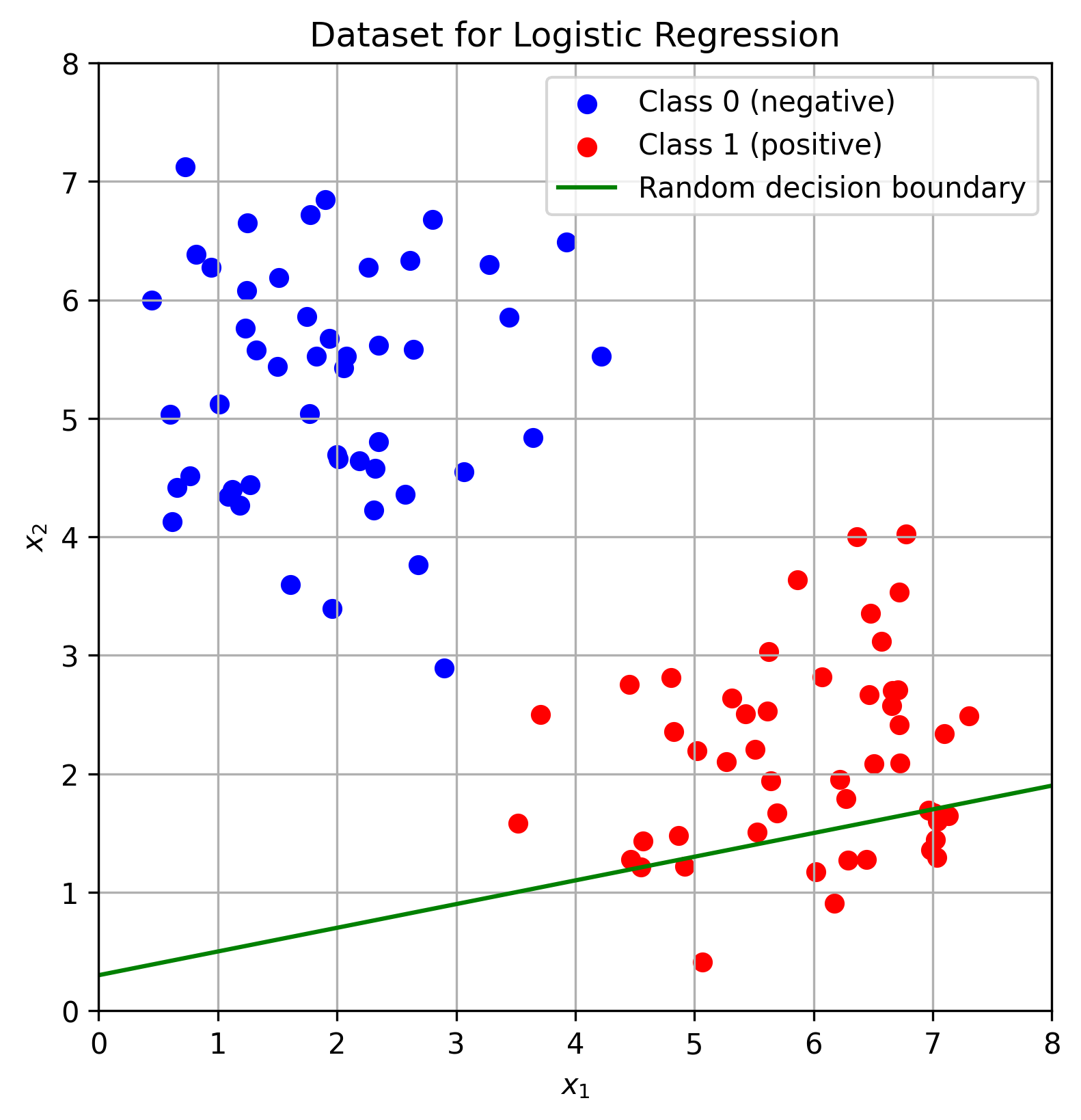
In binary logistic regression we learn a decision boundary that separates points of the negative class (class 0) from those of the positive class (class 1). For a two-dimensional feature space that boundary is a straight line. An example is given below. The green line is a random decision boundary which obviously does not a good job separating the data.

The decision boundary can be described by the following equation:

\[w^T x + b = 0\]

In other words, the decision boundary is the set of points for which $w^T x+b$ equals to zero.

Here $x$ is the input that we provide to the model (i.e. the data point that we want to classify) and $w$ and $b$ are the parameters of the model. In the example above we have two features $x_1$ and $x_2$. Therefore, $w = (w_1, w_2)$ and $x = (x_1, x_2)$ are two dimensional vectors (usually column vectors). The parameter $b$ (the bias) is a scalar. The bias term enables the model to shift the decision boundary away from the origin. Without it, the model would be constrained to decision boundaries that pass through the origin, which may not be suitable for all datasets.

An input belongs to class 0 (or the negative class) if $w^Tx<0$, otherwise it belongs to class 1 (positive class).

For instance, in the example above we have a blue point that is close to (1, 5). The parameters of the model are

\[w = \begin{bmatrix} 0.2 \\ -1.0 \end{bmatrix} \qquad b = 0.3\]

If we compute $w^Tx + b$ for the point $(1,5) with the model’s parameters, we get

\[\begin{bmatrix} 0.2 & -1.0 \end{bmatrix} \begin{bmatrix} 1 \\ 5 \end{bmatrix} + 0.3 = 0.2 \cdot 1 -1\cdot 5 + 0.3 = -4.5\]

Since this value is negative, the point $(1,5)$ belongs to the negative class.

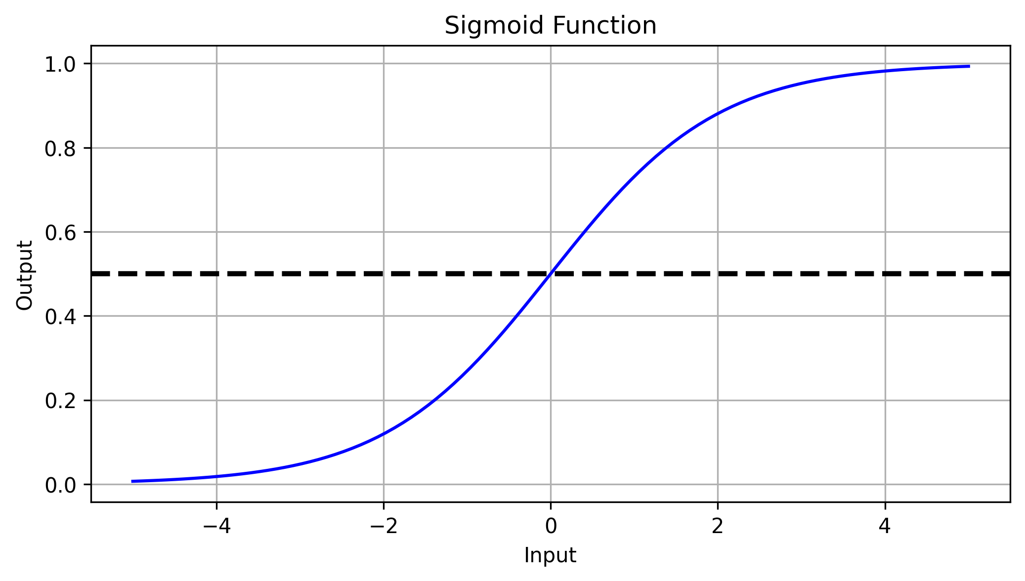
The value of $w^Tx + b$ is also called the logit. Logistic regression converts it to a probability with the sigmoid function. It returns the probability that a given point belongs to the positive class. The sigmoid function is defined as:

\[\sigma(x) = \frac{1}{1 + e^{-x}}\]

If we plot the graph of the sigmoid function we can see that it approaches 0 if the input $x$ goes to $-\infty$ and 1 if the input goes to $\infty$. For $x= 0$ the output is equal to 0.5 which means that for a point $x$ for which $w^Tx+b = 0$, the probability that the point belongs to the positive class is 50%.

To dertermine the probability that a point $x$ belongs to the positive class, logistic regression computes

\[f(x) = \sigma(w^Tx+b) = \frac{1}{1 + e^{-(w^Tx+b)}}\]

Stealing parameters

An adversary who knows how the model computes $f(x)$ but not its parameters can recover the parameters by carefully chosen queries.

Let’s assume the model has the parameters $w^T=(w_1, w_2)$ and $b$. After sending a query $q = (q_1, q_2)$ to the model the adversary knows the value of $f(q)$. Due to

\[f(q) = \sigma(w^Tq+b) = \frac{1}{1 + e^{-(w^Tq+b)}}\]

and after rearranging the terms, the adversary gets the logits for the query:

\[w^Tq + b = -\ln\left(\frac{1}{f(q)} - 1\right)\]

Let’s walk through a concrete example to see how an adversary can determine the parameters of a logistic regression model with two features.

In this example, we assume the model’s parameters are $w = (0.2, -1.0)$ and $b = 0.3$. These parameters are unknown to the adversary.

To infer them, the adversary sends three queries to the model and records the corresponding logits - i.e., the output of the linear function $w^T x + b$.

The first query $q_1 = (1, 5)$ results in a logit of $1\cdot 0.2 - 5\cdot 1 + 0.3 = -4.5$.
The second query $q_2 = (3, 2)$ results in a logit of $-1.1$.
The third query $q_3 = (3, 4)$ results in a logit of $-3.1$.

Using these inputs and outputs, the adversary can now construct a system of linear equations:

\[\begin{bmatrix} 1 & 5 & 1 \\ 3 & 2 & 1 \\ 3 & 4 & 1 \end{bmatrix} \begin{bmatrix} w_1 \\ w_2 \\ b \end{bmatrix} = \begin{bmatrix} -4.5 \\ -1.2 \\ -3.1 \end{bmatrix}\]

This system of equations contains three unknowns: $w_1$, $w_2$, and $b$. Since we also have three equations, the system can be solved exactly.

We could use NumPy to do so:

import numpy as np

Q = np.array([
    [1, 5, 1],
    [3, 2, 1],
    [3, 4, 1]
])
logits = np.array([-4.5, -1.1, -3.1])
np.linalg.solve(Q, logits)

The result is: [0.2, -1.0, 0.3], which exactly matches the parameters of our model. This shows that we were able to recover the model’s parameters using only the responses to our queries.

This approach can, of course, be generalized to any number of parameters. To determine the parameters of a model with $n$ parameters, $n$ queries to the model are sufficient. This yields a system of $n$ equations with $n$ unknowns, which can then be solved.